Integrate Your SAP BW Data in Microsoft Fabric

Summary
This article demonstrates how to integrate SAP BW data in Microsoft Fabric using ERPL, providing a comprehensive guide for connecting enterprise SAP systems to Microsoft's modern data platform.
Why Fabric, Why SAP, Why Together
Microsoft Fabric pulls every Microsoft analytics product — Synapse, Data Factory, Power BI, OneLake — into a single workspace. For organisations already standardised on the Microsoft stack, it's the obvious place to land enterprise data. SAP BW, meanwhile, is where most of that organisation's "official" analytical truth still lives: cubes, queries, lineage, mapping tables, hierarchies.
The gap between the two has historically been wide. Native Fabric connectors for SAP BW exist but are tuned for OData V4 — they don't speak BICS, they don't expose hierarchies cleanly, and they can't traverse query→cube→DataSource lineage. So teams either ship through SAP Datasphere as an intermediate, build a custom Power Query, or pay a third party for a Fabric-SAP adapter.
We took a different route: install ERPL inside a Fabric notebook and let DuckDB do the talking. Same SQL contract end-to-end, no intermediate landing.
The Stack
+--------------+        +-----------------+       +--------+
| SAP BW       | <----> | ERPL (BICS/RFC) | <---> | DuckDB |
+--------------+        +-----------------+       +---+----+
                                                      |
                                                      v
                                                 OneLake / Lakehouse
                                                      |
                                                      v
                                                  Power BI
ERPL runs as a DuckDB extension. A Fabric notebook spins up a Python kernel, installs DuckDB, installs ERPL, configures a SAP secret, and reads BW directly. The result lands in OneLake as Delta or Parquet, and the rest of the Fabric stack — pipelines, semantic models, Power BI reports — consumes it like any other Fabric asset.
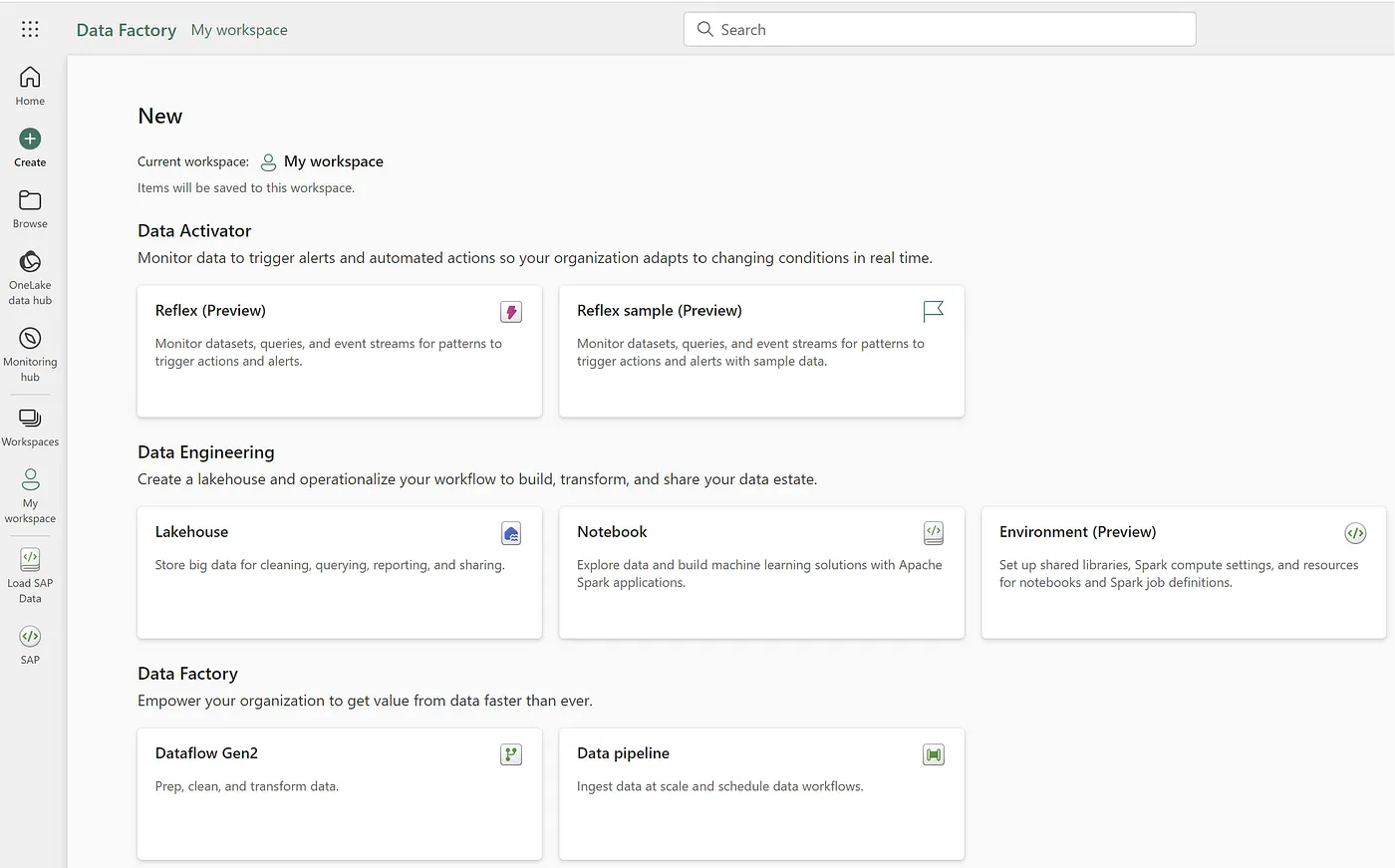
Step 1: Spin Up a Fabric Notebook
Inside your Fabric workspace, create a Notebook and attach it to a Lakehouse.
In the first cell, install DuckDB and load the ERPL extension:
%pip install duckdb

import duckdb
con = duckdb.connect()
con.execute("INSTALL 'erpl' FROM 'http://get.erpl.io';")
con.execute("LOAD 'erpl';")
ERPL is now available in this session. Loading it inside the notebook keeps the SAP credentials scoped to the workspace rather than baked into a pipeline definition.
Step 2: Configure the SAP Connection
Use a DuckDB secret for the SAP credentials. In production you'd source these from a Fabric Key Vault or workspace identity; for a first walkthrough, environment variables work fine:
con.execute("""
CREATE SECRET sap (
  TYPE sap_rfc,
  ASHOST '%s',
  SYSNR  '%s',
  CLIENT '%s',
  USER   '%s',
  PASSWD '%s',
  LANG   'EN'
);
""" % (
    os.environ["SAP_ASHOST"],
    os.environ["SAP_SYSNR"],
    os.environ["SAP_CLIENT"],
    os.environ["SAP_USER"],
    os.environ["SAP_PASSWD"],
))

con.execute("PRAGMA sap_rfc_ping").fetchall()
PRAGMA sap_rfc_ping raises if anything is misconfigured — a one-line connectivity check before you write the rest of the pipeline.
Step 3: Read a BW Query
The interesting part. ERPL's BICS protocol lets you call existing BEx queries with the same selection logic the business users hit them with in Analysis for Office. The composition pattern is begin → filter → result:
df = con.execute("""
SELECT *
FROM sap_bics_result(
  sap_bics_filter(
    sap_bics_begin('ZQ_SALES_2024'),
    '0CALMONTH', '202401'
  )
);
""").fetch_df()

df.head()
The query you call (ZQ_SALES_2024 above) is just the BEx query technical name — the same name your BW team uses in RSRT or in Analysis for Office. Hierarchies, variables, restricted key figures: all evaluated server-side, the same way your BW power users see them. ERPL just streams the resulting cells into a pandas DataFrame.
Step 4: Persist to OneLake
A DataFrame is useful for exploration; for downstream Fabric pipelines you want it in the Lakehouse. Push it to the workspace's default Lakehouse as a Delta table:
# Spark/Delta path from the attached Lakehouse
spark.createDataFrame(df).write \
    .mode("overwrite") \
    .format("delta") \
    .saveAsTable("bw_sales_202401")
That table is now visible in the Lakehouse explorer, queryable from SQL endpoints, and available to every Power BI semantic model in the workspace.
Step 5: Schedule and Forget
The Fabric scheduler can run the notebook on whatever cadence you need — hourly, daily, or triggered by upstream events. Combine it with ERPL's ODP support (instead of BICS) and you can do incremental delta extracts: first scheduled run pulls a full snapshot, every subsequent run pulls only the changes.
# Same pattern with ODP — cursor state lives in SAP, no per-call mode flag
df = con.execute(
    "SELECT * FROM sap_odp_read_full('BW', 'VBAK$F', threads => 4);"
).fetch_df()
First call: FULL. Every subsequent call: DELTA. The Fabric notebook does nothing special — SAP tracks the cursor.
What This Replaces
A typical "SAP BW → Fabric" pipeline used to involve three or four moving parts: a scheduled SAP job exporting to file, a Data Factory pipeline pulling that file into OneLake, a Spark notebook cleaning it, a semantic model consuming it. Each handoff adds latency and breakage surface.
With ERPL inside the notebook, the pipeline collapses to one stage. Latency drops from "tomorrow morning's data is available by 10 AM" to "current data is available the moment the notebook runs". And because everything flows through DuckDB SQL, the same pipeline definition you write for an ad-hoc exploration also works as the scheduled production job — no rewriting between modes.
Where to Go From Here
- Install ERPL — the prerequisite for everything above.
- BICS Protocol Deep Dive — full reference for the
sap_bics_*family, including hierarchies and lineage. - ODP Protocol Deep Dive — cursor-state delta extraction.
- Book a demo if you want us to walk through the Fabric integration with your own BW system in front of you.
The Microsoft side of the integration is documented thoroughly in the Fabric docs; the only new piece is the ERPL line at the start of your notebook. Everything else is the standard Fabric flow.