Your SAP Data Is Already Real-Time — You Just Need to Stop Caching It

Picture a forecasting team at an industrial-controls Mittelstand. Their job for the next quarter: launch an AI-driven inventory and demand-forecasting tool that the operations team will actually trust enough to act on. They have the model. They have the GPUs. They cannot ship.
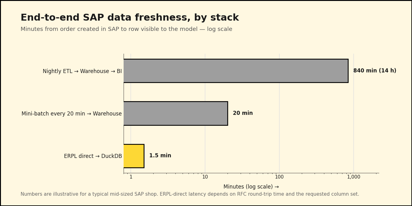
The reason: their nightly ETL job runs at 02:00 and finishes around 04:00, by which point the model trains on data that's already half a day old. By the time the forecast reaches the procurement system at 08:00, it's reasoning about a world that existed fourteen hours ago. When the CFO asks why the model recommended ordering more of an item that just sold out at lunchtime, nobody has a good answer — because the data the model saw never knew the lunchtime existed.
The fix isn't a better ETL. The fix is removing the ETL.
Why "real-time" usually means "20 minutes ago"
The default SAP analytics architecture is three boxes: SAP, a warehouse, a BI layer on top of the warehouse. Each box exists because someone, at some point, decided the next box couldn't talk to the previous one directly. That assumption was true in 2008. It's been getting less true every year since DuckDB shipped.
When you actually trace the latency, the SAP system isn't the slow part. RFC reads on a healthy ECC system come back in seconds. ODP delta extracts on a properly subscribed data source return whatever changed since the last cursor position, often in under a minute. The latency lives in the middle box — the warehouse you assumed you needed because everyone else has one.
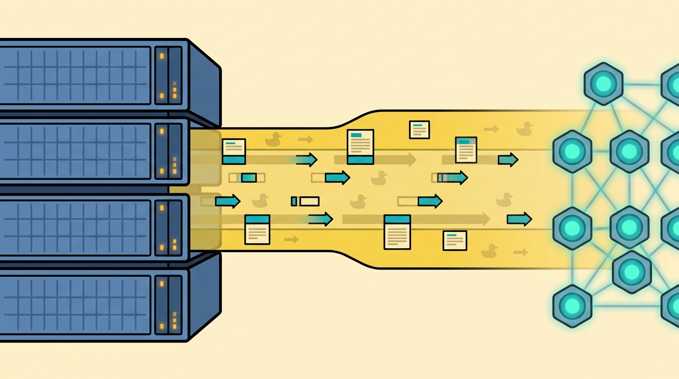
What if you didn't have one? What if your AI agents and your forecasting models queried SAP through a thin SQL layer that fans out to RFC, ODP, Datasphere, and Business Central — and only materialized when it actually helped? That's the stack we built ERPL for.

Layer 1: ERPL pulls SAP ECC / S/4HANA live
The starting point is a DuckDB secret. ERPL stores SAP credentials the same way DuckDB stores S3 or Postgres credentials — once, declaratively, with the connection metadata attached. From then on, every ERPL function uses the secret implicitly.
INSTALL 'erpl' FROM 'http://get.erpl.io';
LOAD 'erpl';

CREATE SECRET sap (
  TYPE sap_rfc,
  ASHOST 'sap-prod.example.com',
  SYSNR  '00',
  CLIENT '100',
  USER   'erpl_reader',
  PASSWD 'redacted',
  LANG   'EN'
);

PRAGMA sap_rfc_ping;
PRAGMA sap_rfc_ping raises immediately if anything is misconfigured, so the credentials check is one statement, not a 200-line connection class.
With the secret in place, you read SAP tables as if they were DuckDB tables — including pushdown for WHERE and column selection. The forecasting team needs recent sales-order headers (VBAK) for one of their sales organizations. ERPL's sap_read_table has predicate pushdown enabled, so a regular SQL WHERE clause is pushed all the way down into the RFC call. You don't write a special filter parameter; you write SQL:
SELECT VBELN, ERDAT, KUNNR, NETWR, WAERK
FROM sap_read_table('VBAK', MAX_ROWS => 5000)
WHERE ERDAT >= DATE '2026-05-01'
  AND VKORG = '1000';
That executes in seconds against a live ECC instance. The MAX_ROWS is a guardrail; pushdown narrows the read further. For column-heavy tables you can also pass COLUMNS => ['VBELN', 'ERDAT', 'KUNNR'] and let RFC drop the rest before bytes leave SAP.
For incremental loads, RFC is the wrong tool — that's what ODP is for. ODP cursors are server-side state: SAP remembers what you've already seen per subscriber. The first call to sap_odp_read_full for a given (context, data source) returns a FULL snapshot and opens the cursor. Every subsequent call returns only the DELTA since the last position. There is no per-call mode flag and no manual cursor management — the server tracks it.
-- First call: SAP returns the full snapshot and opens the cursor.
-- Every subsequent call: only the delta since the last position.
SELECT *
FROM sap_odp_read_full('BW', 'VBAK$F', threads => 4);
Run that on a cron every few minutes and you have a continuously-fresh sales-order stream landing directly in DuckDB, with zero ETL code between SAP and your model.
Layer 2: ERPL-Web closes the cloud gap
Not every SAP system is on-prem. Some of the forecasting team's data lives in Microsoft Dynamics 365 Business Central (the spin-off subsidiary uses BC instead of S/4HANA), and the corporate planning numbers are in SAP Datasphere. We built ERPL-Web so the same DuckDB session can reach both without changing the SQL contract.
For Business Central, attach the company as if it were a database:
INSTALL 'erpl_web' FROM 'http://get.erpl.io';
LOAD 'erpl_web';

ATTACH 'CRONUS Germany AG' AS bc (TYPE business_central);

-- Now the BC entities look like regular tables
SELECT no, name, balance_due
FROM bc.customer
WHERE balance_due > 0
ORDER BY balance_due DESC
LIMIT 20;
ATTACH does the OData V4 metadata discovery once. After that, every entity in the company shows up as a DuckDB table, with predicate pushdown via the OData $filter clause.
For Datasphere, the read function speaks the same SQL dialect:
SELECT *
FROM datasphere_read_relational('PLANNING_SPACE', 'V_DEMAND_FORECAST')
WHERE month = '2026-05';
The forecasting team doesn't care that one read goes through SAP-managed OAuth2 and the other goes through RFC over an SSH tunnel. Same SELECT *, same DuckDB result set. That uniformity is what lets the data plane disappear.
Layer 3: anofox-tabular gates the stream
Live data is fast, but live data is also dirty. The forecasting model needs the dirty rows filtered out before it sees them, not flagged in a Monday-morning report. anofox-tabular is a DuckDB extension that runs the validation in SQL, vectorized, in-process — no external service call, no Python ML pipeline.
Take the customer master. Two checks the team runs every load: are the customer email addresses syntactically valid, and are the German VAT numbers well-formed for the country they claim? Emails live in ADR6, joined to KNA1 via ADRNR, so the pattern is one CTE plus two calls:
LOAD anofox_tabular;

WITH customers AS (
  SELECT k.KUNNR, k.NAME1, k.LAND1, k.STCEG, e.SMTP_ADDR
  FROM sap_read_table('KNA1') AS k
  LEFT JOIN sap_read_table('ADR6') AS e
    ON e.ADDRNUMBER = k.ADRNR
  WHERE k.LAND1 = 'DE'
)
SELECT KUNNR, NAME1, SMTP_ADDR, STCEG
FROM customers
WHERE NOT email_is_valid(SMTP_ADDR)
   OR NOT vat_is_valid(STCEG, 'DE');
That returns the rows that failed validation — perfect for an alert table the data steward gets pinged on.
The more interesting catch is statistical. The forecasting model trains on order line values and quantities. A single rogue row — wrong net value for the quantity, or vice versa — can knock the model's RMSE up by an order of magnitude. anofox-tabular's isolation forest works directly against a DuckDB table:
-- Persist the last week of orders so isolation_forest_mv can reference it by name
CREATE OR REPLACE TABLE live_orders AS
SELECT VBELN, POSNR, KDGRP, NETWR, KWMENG
FROM sap_odp_read_full('BW', 'VBAP$F')
WHERE ERDAT >= CURRENT_DATE - INTERVAL '7' DAY;

-- Multi-column isolation forest. Positional args:
--   (table_name, columns_csv, n_trees, sample_size, contamination, output_mode)
SELECT row_id, anomaly_score
FROM isolation_forest_mv(
  'live_orders', 'NETWR,KWMENG',
  100, 256, 0.005, 'scores'
)
WHERE is_anomaly
ORDER BY anomaly_score DESC
LIMIT 20;
The first time we ran this against the Mittelstand's pre-production cutover data, the top anomaly was a single order line whose NETWR was a thousand times too large for its KWMENG — a unit-mismatch from a legacy ABAP report. Joining the row_id back to live_orders revealed the offending row also carried KDGRP = '9999', a placeholder value the same report had been writing for years. The forecasting model would have eaten both surprises without complaint and quietly skewed every prediction for that segment.
What this looks like in production
You don't need a Kafka cluster for this. The whole stack runs in one DuckDB process. A typical hourly job:
-- 1. Pull the delta (advances the ODP cursor once)
CREATE OR REPLACE TABLE orders_hourly AS
SELECT *
FROM sap_odp_read_full('BW', 'VBAP$F');

-- 2. Score for anomalies (runs against the snapshot, not the cursor)
CREATE OR REPLACE TABLE orders_flagged AS
SELECT *
FROM isolation_forest_mv(
  'orders_hourly', 'NETWR,KWMENG',
  100, 256, 0.005, 'scores'
);

-- 3. Hand the clean rows to the model
CREATE OR REPLACE VIEW forecast_inputs AS
SELECT o.*
FROM orders_hourly AS o
LEFT JOIN orders_flagged AS f ON f.row_id = o.rowid
WHERE f.is_anomaly IS NOT TRUE;
Persist orders_hourly and orders_flagged through DuckLake snapshots if you want time-travel or audit. Latency budget on this stack against a real ECC system: under 90 seconds for an RFC table read, under 5 minutes for an ODP delta load that captures a quarter-day of order activity. No warehouse landing, no staging tables, no nightly window.
Next week, in Part 2
We have a fresh, validated view of SAP reality. The forecasting model could already train on it, and the dashboards could already read it. But there's a second consumer the team hasn't onboarded yet: the AI agent that's supposed to use this data — and, occasionally, write back to SAP when it notices something wrong. That's where flAPI and erpl-adt come in.